上次说到的,使用如下代码保存矢量图时,放在外侧的图例往往显示不完整:
import numpy as np
import matplotlib.pyplot as plt
fig, ax = plt.subplots()
x1 = np.random.uniform(-10, 10, size=20)
x2 = np.random.uniform(-10, 10, size=20)
#print(x1)
#print(x2)
number = []
x11 = []
x12 = []
for i in range(20):
  number.append(i+1)
  x11.append(i+1)
  x12.append(i+1)
plt.figure(1)
# you can specify the marker size two ways directly:
plt.plot(number, x1, 'bo', markersize=20,label='a') # blue circle with size 20
plt.plot(number, x2, 'ro', ms=10,label='b') # ms is just an alias for markersize

lgnd=plt.legend(bbox_to_anchor=(1.05, 1), loc=2, borderaxespad=0,numpoints=1,fontsize=10)
lgnd.legendHandles[0]._legmarker.set_markersize(16)
lgnd.legendHandles[1]._legmarker.set_markersize(10)

plt.show()

fig.savefig('scatter.png',dpi=600)
保存为scatter.png之后的效果为:

可以看到放在图像右上的图例只显示了左边一小部分。
这里的原因很简单,使用savefig()函数进行保存矢量图时,它是通过一个bounding box (bbox, 边界框),进行范围的框定,只将落入该框中的图像进行保存,如果图例没有完全落在该框中,自然不能被保存。
懂得了其原理,再进行解决问题就比较简单了。
这里有两个解决思想:
1. 将没有完全落入该bbox的图像,通过移动的方法,使其完全落入该框中,那么bbox截取的图像即是完整的 (将图像移入bbox中);
2. 改变bbox的大小,使其完全包含该图像,尤其是往往落入bbox外侧的图例 (将bbox扩大到完全包含图像)。
下面分别介绍基于这两个思想解决这个问题的两种方法:
1. 利用函数subplots_adjust()
在该官方文档中可以看到,subplots_adjust()函数的作用是调整子图布局,它包含6个参数,其中4个参数left, right, bottom, top的作用是分别调整子图的左部,右部,底部,顶部的位置,另外2个参数wspace, hspace的作用分别是调整子图之间的左右之间距离和上下之间距离。
其默认数值分别为:
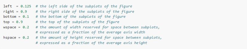
以上述图为例,现考虑既然图例右侧没有显示,则调整subplots_adjust()函数的right参数,使其位置稍往左移,将参数right默认的数值0.9改为0.8,那么可以得到一个完整的图例:
import numpy as np
import matplotlib.pyplot as plt
fig, ax = plt.subplots()
x1 = np.random.uniform(-10, 10, size=20)
x2 = np.random.uniform(-10, 10, size=20)
#print(x1)
#print(x2)
number = []
x11 = []
x12 = []
for i in range(20):
  number.append(i+1)
  x11.append(i+1)
  x12.append(i+1)
plt.figure(1)
# you can specify the marker size two ways directly:
plt.plot(number, x1, 'bo', markersize=20,label='a') # blue circle with size 20
plt.plot(number, x2, 'ro', ms=10,label='b') # ms is just an alias for markersize

lgnd=plt.legend(bbox_to_anchor=(1.05, 1), loc=2, borderaxespad=0,numpoints=1,fontsize=10)
lgnd.legendHandles[0]._legmarker.set_markersize(16)
lgnd.legendHandles[1]._legmarker.set_markersize(10)

fig.subplots_adjust(right=0.8)

plt.show()

fig.savefig('scatter1.png',dpi=600)
保存为scatter1.png之后和scatter.png的对比效果为:

可以看到这时scatter1.png的图例显示完整,它是通过图像的右侧位置向左移动而被整体包含在保存的图像中完成的。
同理,若legend的位置在图像下侧,使用savefig()保存时也是不完整的,这时需要修改的是函数subplots_adjust()的参数bottom,使其向上移,而被包含在截取图像进行保存的框中,即下文介绍的bbox。
import numpy as np import matplotlib.pyplot as plt fig, ax = plt.subplots() x1 = np.random.uniform(-10, 10, size=20) x2 = np.random.uniform(-10, 10, size=20) #print(x1) #print(x2) number = [] x11 = [] x12 = [] for i in range(20): number.append(i+1) x11.append(i+1) x12.append(i+1) plt.figure(1) # you can specify the marker size two ways directly: plt.plot(number, x1, 'bo', markersize=20,label='a') # blue circle with size 20 plt.plot(number, x2, 'ro', ms=10,label='b') # ms is just an alias for markersize lgnd=plt.legend(bbox_to_anchor=(0.4, -0.1), loc=2, borderaxespad=0,numpoints=1,fontsize=10) lgnd.legendHandles[0]._legmarker.set_markersize(16) lgnd.legendHandles[1]._legmarker.set_markersize(10) plt.show() fig.savefig('scatter#1.png',dpi=600)由于subplots_adjust()中默认的bottom值为0.1,故添加fig.subplots_adjust(bottom=0.2),使其底部上移,修改为
import numpy as np
import matplotlib.pyplot as plt
fig, ax = plt.subplots()
x1 = np.random.uniform(-10, 10, size=20)
x2 = np.random.uniform(-10, 10, size=20)
#print(x1)
#print(x2)
number = []
x11 = []
x12 = []
for i in range(20):
  number.append(i+1)
  x11.append(i+1)
  x12.append(i+1)
plt.figure(1)
# you can specify the marker size two ways directly:
plt.plot(number, x1, 'bo', markersize=20,label='a') # blue circle with size 20
plt.plot(number, x2, 'ro', ms=10,label='b') # ms is just an alias for markersize

lgnd=plt.legend(bbox_to_anchor=(0.4, -0.1), loc=2, borderaxespad=0,numpoints=1,fontsize=10)
lgnd.legendHandles[0]._legmarker.set_markersize(16)
lgnd.legendHandles[1]._legmarker.set_markersize(10)

fig.subplots_adjust(bottom=0.2)

plt.show()
fig.savefig('scatter#1.png',dpi=600)
效果对比:
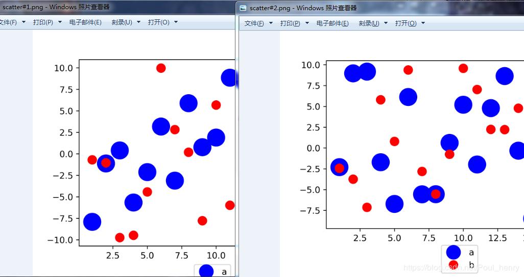
图例legend在其它位置同理。
2. 利用函数savefig()
上个博客讲到,使用savefig()函数中的三个参数fname, dpi, format可用以保存矢量图,现用该函数中另一个参数bbox_inches使
未保存到图中的图例包含进来。
下图可以看到,bbox_inches的作用是调整图的bbox, 即bounding box(边界框)
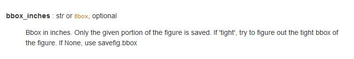
可以看到,当bbox_inches设为'tight'时,它会计算出距该图像的较紧(tight)边界框bbox,并将该选中的框中的图像保存。
这里的较紧的边界框应该是指完全包含该图像的一个矩形,但和图像有一定的填充距离,和Minimum bounding box(最小边界框),个人认为,有一定区别。单位同样是英寸(inch)。
这样图例就会被bbox包含进去,进而被保存。
完整代码:
import numpy as np
import matplotlib.pyplot as plt
fig, ax = plt.subplots()
x1 = np.random.uniform(-10, 10, size=20)
x2 = np.random.uniform(-10, 10, size=20)
#print(x1)
#print(x2)
number = []
x11 = []
x12 = []
for i in range(20):
  number.append(i+1)
  x11.append(i+1)
  x12.append(i+1)
plt.figure(1)
# you can specify the marker size two ways directly:
plt.plot(number, x1, 'bo', markersize=20,label='a') # blue circle with size 20
plt.plot(number, x2, 'ro', ms=10,label='b') # ms is just an alias for markersize

lgnd=plt.legend(bbox_to_anchor=(1.05, 1), loc=2, borderaxespad=0,numpoints=1,fontsize=10)
lgnd.legendHandles[0]._legmarker.set_markersize(16)
lgnd.legendHandles[1]._legmarker.set_markersize(10)

#fig.subplots_adjust(right=0.8)

plt.show()

fig.savefig('scatter2.png',dpi=600,bbox_inches='tight')
保存为scatter2.png,下面是scatter.png, scatter1.png, scatter2.png三张图的对比:
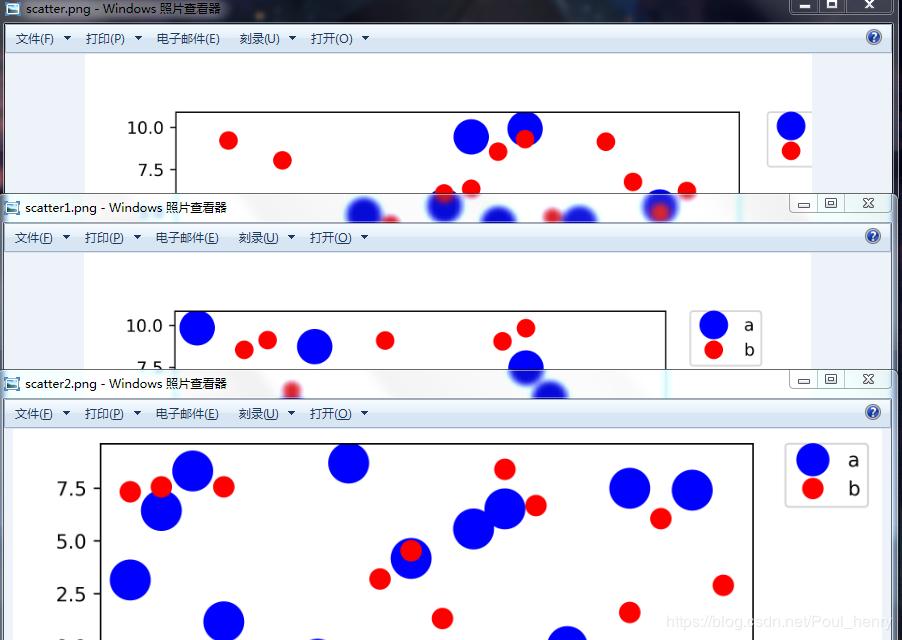
可以看到,scatter1.png,即第1种方法的思想,是将图像的右侧边界向左移动,截取该图用以保存的bbox未变;而scatter2.png,即第2种方法的思想,是直接将截取该图用以保存的bbox扩大为整个图像,而将其全部包括。
注:savefig()还有两个参数需要说明
其中一个是pad_inches,它的作用是当前面的bbox_inches为'tight'时,调整图像和bbox之间的填充距离,这里不需要设置,只要选择默认值即可。

个人认为,如果设置pad_inches参数为0,即pad_inches=0,截取图进行保存的bbox就是minimum bounding box (最小边界框)。
另外一个是bbox_extra_artists,它的作用是计算图像的bbox时,将其它的元素也包含进去。

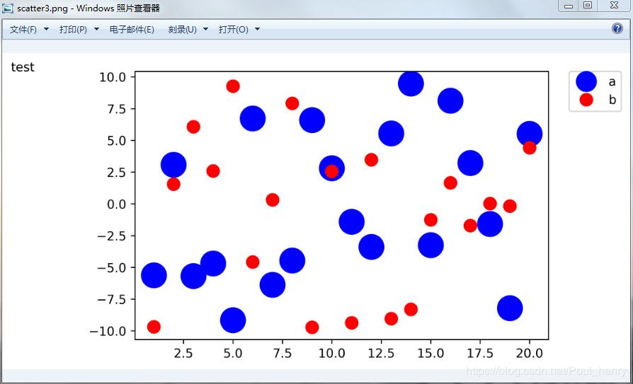
这里举个例子,如果在图像左侧再加一个文本框text,保存图像时希望该文本框包含在bbox中,则可以使用该参数bbox_extra_artists将text包含进去(实际使用中,即使未使用bbox_extra_artists,保存的图像也包含该text):
import numpy as np
import matplotlib.pyplot as plt
fig, ax = plt.subplots()
x1 = np.random.uniform(-10, 10, size=20)
x2 = np.random.uniform(-10, 10, size=20)
#print(x1)
#print(x2)
number = []
x11 = []
x12 = []
for i in range(20):
  number.append(i+1)
  x11.append(i+1)
  x12.append(i+1)
plt.figure(1)
# you can specify the marker size two ways directly:
plt.plot(number, x1, 'bo', markersize=20,label='a') # blue circle with size 20
plt.plot(number, x2, 'ro', ms=10,label='b') # ms is just an alias for markersize

lgnd=plt.legend(bbox_to_anchor=(1.05, 1), loc=2, borderaxespad=0,numpoints=1,fontsize=10)
lgnd.legendHandles[0]._legmarker.set_markersize(16)
lgnd.legendHandles[1]._legmarker.set_markersize(10)

text = ax.text(-0.3,1, "test", transform=ax.transAxes)

#fig.subplots_adjust(right=0.8)
plt.show()
fig.savefig('scatter3.png',dpi=600, bbox_extra_artists=(lgnd,text),bbox_inches='tight')
显示效果:
为防止有的元素没有被包含在bbox中,可以考虑使用该参数
到此这篇关于Python matplotlib图例放在外侧保存时显示不完整问题解决的文章就介绍到这了,更多相关matplotlib外侧保存显示不完整内容请搜索python博客以前的文章或继续浏览下面的相关文章希望大家以后多多支持python博客!
-
<< 上一篇 下一篇 >>
标签:numpy matplotlib
Python matplotlib图例放在外侧保存时显示不完整问题解决
看: 2049次 时间:2020-08-22 分类 : 数据分析
- 相关文章
- 2021-12-20python数据挖掘使用Evidently创建机器学习模型仪表板
- 2021-12-20Python多进程共享numpy 数组的方法
- 2021-12-20python数据分析近年比特币价格涨幅趋势分布
- 2021-12-20python调用matlab的方法详解
- 2021-12-20python学习与数据挖掘应知应会的十大终端命令
- 2021-07-20pandas中NaN缺失值的处理方法
- 2021-07-20Python数据分析入门之数据读取与存储
- 2021-07-20Python 如何读取字典的所有键-值对
- 2021-07-20如何获取numpy的第一个非0元素索引
- 2021-07-20Python机器学习之KNN近邻算法
-
搜索
-
-
推荐资源
-
Powered By python教程网 鲁ICP备18013710号
python博客 - 小白学python最友好的网站!