1. 多曲线

1.1 使用pyplot方式

import numpy as np
import matplotlib.pyplot as plt

x = np.arange(1, 11, 1)

plt.plot(x, x * 2, label="First")
plt.plot(x, x * 3, label="Second")
plt.plot(x, x * 4, label="Third")

plt.legend(loc=0, ncol=1)  # 参数：loc设置显示的位置，0是自适应；ncol设置显示的列数

plt.show()

1.2 使用面向对象方式

import numpy as np
import matplotlib.pyplot as plt

x = np.arange(1, 11, 1)

fig = plt.figure()
ax = fig.add_subplot(111)


ax.plot(x, x * 2, label="First")
ax.plot(x, x * 3, label="Second")

ax.legend(loc=0)
# ax.plot(x, x * 2)
# ax.legend([”Demo“], loc=0)

plt.show()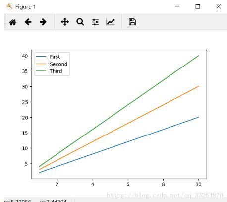

2. 双y轴曲线

双y轴曲线图例合并是一个棘手的操作，现以MNIST案例中loss/accuracy绘制曲线。

import tensorflow as tf
from tensorflow.examples.tutorials.mnist import input_data
import time
import matplotlib.pyplot as plt
import numpy as np

x_data = tf.placeholder(tf.float32, [None, 784])
y_data = tf.placeholder(tf.float32, [None, 10])
x_image = tf.reshape(x_data, [-1, 28, 28, 1])

# convolve layer 1
filter1 = tf.Variable(tf.truncated_normal([5, 5, 1, 6]))
bias1 = tf.Variable(tf.truncated_normal([6]))
conv1 = tf.nn.conv2d(x_image, filter1, strides=[1, 1, 1, 1], padding='SAME')
h_conv1 = tf.nn.sigmoid(conv1 + bias1)
maxPool2 = tf.nn.max_pool(h_conv1, ksize=[1, 2, 2, 1], strides=[1, 2, 2, 1], padding='SAME')

# convolve layer 2
filter2 = tf.Variable(tf.truncated_normal([5, 5, 6, 16]))
bias2 = tf.Variable(tf.truncated_normal([16]))
conv2 = tf.nn.conv2d(maxPool2, filter2, strides=[1, 1, 1, 1], padding='SAME')
h_conv2 = tf.nn.sigmoid(conv2 + bias2)
maxPool3 = tf.nn.max_pool(h_conv2, ksize=[1, 2, 2, 1], strides=[1, 2, 2, 1], padding='SAME')

# convolve layer 3
filter3 = tf.Variable(tf.truncated_normal([5, 5, 16, 120]))
bias3 = tf.Variable(tf.truncated_normal([120]))
conv3 = tf.nn.conv2d(maxPool3, filter3, strides=[1, 1, 1, 1], padding='SAME')
h_conv3 = tf.nn.sigmoid(conv3 + bias3)

# full connection layer 1
W_fc1 = tf.Variable(tf.truncated_normal([7 * 7 * 120, 80]))
b_fc1 = tf.Variable(tf.truncated_normal([80]))
h_pool2_flat = tf.reshape(h_conv3, [-1, 7 * 7 * 120])
h_fc1 = tf.nn.sigmoid(tf.matmul(h_pool2_flat, W_fc1) + b_fc1)

# full connection layer 2
W_fc2 = tf.Variable(tf.truncated_normal([80, 10]))
b_fc2 = tf.Variable(tf.truncated_normal([10]))
y_model = tf.nn.softmax(tf.matmul(h_fc1, W_fc2) + b_fc2)

cross_entropy = - tf.reduce_sum(y_data * tf.log(y_model))

train_step = tf.train.GradientDescentOptimizer(1e-3).minimize(cross_entropy)

sess = tf.InteractiveSession()
correct_prediction = tf.equal(tf.argmax(y_data, 1), tf.argmax(y_model, 1))
accuracy = tf.reduce_mean(tf.cast(correct_prediction, "float"))
sess.run(tf.global_variables_initializer())

mnist = input_data.read_data_sets("MNIST_data/", one_hot=True)

fig_loss = np.zeros([1000])
fig_accuracy = np.zeros([1000])

start_time = time.time()
for i in range(1000):
  batch_xs, batch_ys = mnist.train.next_batch(200)
  if i % 100 == 0:
    train_accuracy = sess.run(accuracy, feed_dict={x_data: batch_xs, y_data: batch_ys})
    print("step %d, train accuracy %g" % (i, train_accuracy))
    end_time = time.time()
    print("time:", (end_time - start_time))
    start_time = end_time
    print("********************************")
  train_step.run(feed_dict={x_data: batch_xs, y_data: batch_ys})
  fig_loss[i] = sess.run(cross_entropy, feed_dict={x_data: batch_xs, y_data: batch_ys})
  fig_accuracy[i] = sess.run(accuracy, feed_dict={x_data: batch_xs, y_data: batch_ys})
print("test accuracy %g" % sess.run(accuracy, feed_dict={x_data: mnist.test.images, y_data: mnist.test.labels}))


# 绘制曲线
fig, ax1 = plt.subplots()
ax2 = ax1.twinx()
lns1 = ax1.plot(np.arange(1000), fig_loss, label="Loss")
# 按一定间隔显示实现方法
# ax2.plot(200 * np.arange(len(fig_accuracy)), fig_accuracy, 'r')
lns2 = ax2.plot(np.arange(1000), fig_accuracy, 'r', label="Accuracy")
ax1.set_xlabel('iteration')
ax1.set_ylabel('training loss')
ax2.set_ylabel('training accuracy')
# 合并图例
lns = lns1 + lns2
labels = ["Loss", "Accuracy"]
# labels = [l.get_label() for l in lns]
plt.legend(lns, labels, loc=7)
plt.show()

注：数据集保存在MNIST_data文件夹下

其实就是三步：

1）分别定义loss/accuracy一维数组

fig_loss = np.zeros([1000])
fig_accuracy = np.zeros([1000])
# 按间隔定义方式：fig_accuracy = np.zeros(int(np.ceil(iteration / interval)))

2）填充真实数据

 fig_loss[i] = sess.run(cross_entropy, feed_dict={x_data: batch_xs, y_data: batch_ys})
 fig_accuracy[i] = sess.run(accuracy, feed_dict={x_data: batch_xs, y_data: batch_ys})

3）绘制曲线

fig, ax1 = plt.subplots()
ax2 = ax1.twinx()
lns1 = ax1.plot(np.arange(1000), fig_loss, label="Loss")
# 按一定间隔显示实现方法
# ax2.plot(200 * np.arange(len(fig_accuracy)), fig_accuracy, 'r')
lns2 = ax2.plot(np.arange(1000), fig_accuracy, 'r', label="Accuracy")
ax1.set_xlabel('iteration')
ax1.set_ylabel('training loss')
ax2.set_ylabel('training accuracy')
# 合并图例
lns = lns1 + lns2
labels = ["Loss", "Accuracy"]
# labels = [l.get_label() for l in lns]
plt.legend(lns, labels, loc=7)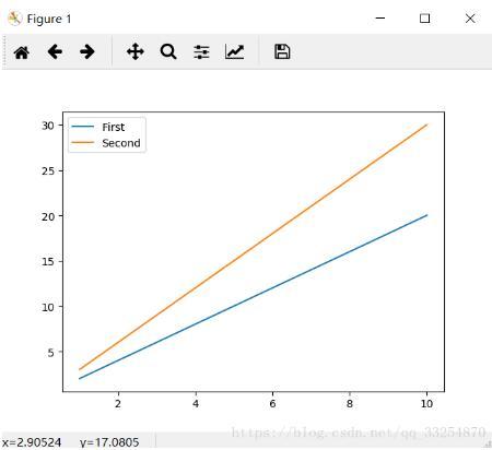

以上这篇TensorFlow绘制loss/accuracy曲线的实例就是小编分享给大家的全部内容了，希望能给大家一个参考，也希望大家多多支持python博客。